
Particle Size Distribution, Mesh Conversion and D10/D50/D90
Mesh number is not a universal particle size. Therefore, industrial buyers should specify the aperture, test method, distribution basis, dispersion procedure and acceptance limits. This guide explains sieve analysis, laser diffraction, D10, D50, D90 and practical mesh-to-micrometre conversion for mineral procurement.
Article navigationWhy particle size matters
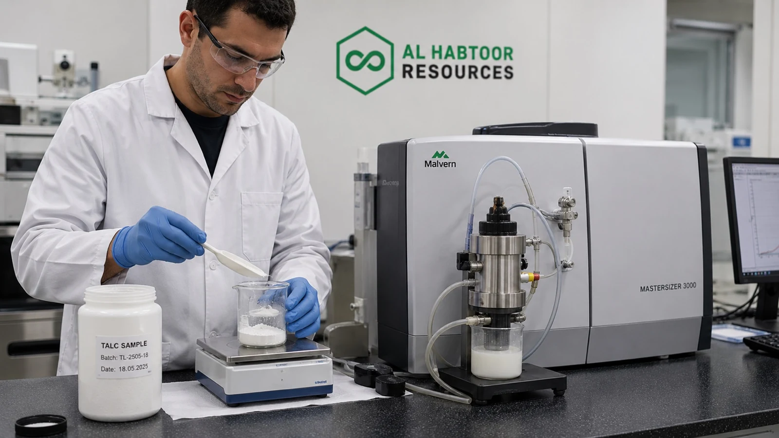
For procurement, the useful question is not simply “What mesh is the powder?” Instead, ask: “Which method measured the distribution, what size basis did it report, and does the result match our process requirement?”
Why particle size matters in industrial minerals
Particle size distribution influences flow, packing, surface area, dispersion, opacity, abrasion and processing behaviour. For example, fine talc can improve surface finish and reinforcement in polymers, while excessive coarse particles may create visible defects or increase screen residue. Likewise, an ore or concentrate with uncontrolled fines may handle differently during loading, drying or downstream processing.
However, one average value cannot describe the whole distribution. A powder may contain the same median size as another lot but a wider coarse tail, more fines or a different particle shape. Therefore, procurement teams should review distribution data rather than approve material from one mesh label or one mean diameter.
Mesh number is not the same as aperture size
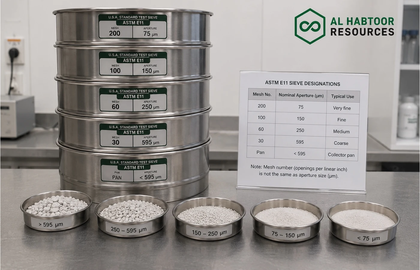
Mesh commonly refers to the number of openings per linear inch in woven wire cloth. Nevertheless, wire diameter also occupies space. As a result, mesh number alone does not define the opening unless the buyer also knows the sieve standard and construction.
For procurement documents, use the nominal aperture in millimetres or micrometres alongside the sieve designation. In addition, state the applicable standard, such as ASTM E11. ASTM E11-24 covers woven wire test sieve cloth and test sieve construction across a nominal aperture range from 125 millimetres down to 20 micrometres.
Do not calculate aperture by dividing 25.4 millimetres by the mesh number. That shortcut ignores wire diameter and can produce a misleading result.
Common ASTM mesh and aperture conversion table
The table below provides common ASTM sieve designations. Use it as a procurement reference, not as a substitute for the current standard or a material-specific test method.
| ASTM sieve number | Nominal aperture | Nominal aperture in micrometres | Typical reporting language |
|---|---|---|---|
| No. 4 | 4.75 mm | 4750 um | Passing 4.75 mm sieve |
| No. 8 | 2.36 mm | 2360 um | Passing 2.36 mm sieve |
| No. 10 | 2.00 mm | 2000 um | Passing 2.00 mm sieve |
| No. 16 | 1.18 mm | 1180 um | Passing 1.18 mm sieve |
| No. 20 | 850 um | 850 um | Passing 850 um sieve |
| No. 30 | 600 um | 600 um | Passing 600 um sieve |
| No. 40 | 425 um | 425 um | Passing 425 um sieve |
| No. 50 | 300 um | 300 um | Passing 300 um sieve |
| No. 60 | 250 um | 250 um | Passing 250 um sieve |
| No. 70 | 212 um | 212 um | Passing 212 um sieve |
| No. 80 | 180 um | 180 um | Passing 180 um sieve |
| No. 100 | 150 um | 150 um | Passing 150 um sieve |
| No. 120 | 125 um | 125 um | Passing 125 um sieve |
| No. 140 | 106 um | 106 um | Passing 106 um sieve |
| No. 170 | 90 um | 90 um | Passing 90 um sieve |
| No. 200 | 75 um | 75 um | Passing 75 um sieve |
| No. 230 | 63 um | 63 um | Passing 63 um sieve |
| No. 270 | 53 um | 53 um | Passing 53 um sieve |
| No. 325 | 45 um | 45 um | Passing 45 um sieve |
| No. 400 | 38 um | 38 um | Passing 38 um sieve |
In practice, suppliers may also use Tyler mesh designations or local standards. Therefore, always confirm the system before converting a commercial label into an aperture value.
How to read D10, D50 and D90
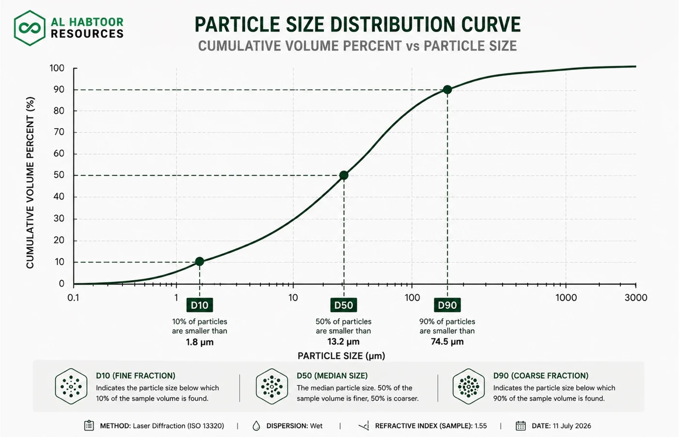
D-values describe points on a cumulative particle size distribution. For a volume-based result, D10 means that 10 percent of the measured particle volume lies below that size. D50 is the median size, while D90 means that 90 percent lies below the reported size.
However, D-values are incomplete without the distribution basis. Laser diffraction commonly reports a volume-equivalent distribution, while imaging or counting methods may report number-based data. Since a small number of coarse particles can dominate volume, the two bases can look very different.
Sieve analysis, laser diffraction and imaging
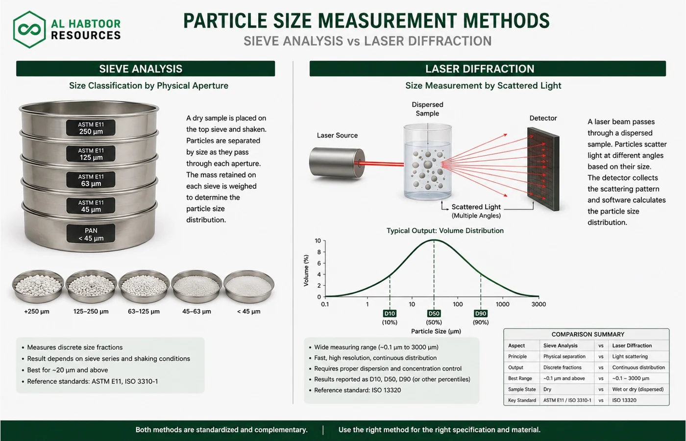
No single method suits every powder. Instead, select the technique according to the size range, particle shape, dispersion behaviour and buyer decision.
| Method | What it measures | Strength | Main limitation |
|---|---|---|---|
| Dry or wet sieving | Mass retained or passing defined apertures | Direct control of coarse fractions and screen residue | Fine, cohesive or plate-like particles may blind sieves or pass according to orientation |
| Laser diffraction | Equivalent particle size from a light-scattering model | Fast, broad distribution and repeatable D-values when dispersion is controlled | Results depend on optical model, dispersion and particle-shape assumptions |
| Dynamic image analysis | Projected particle dimensions and shape descriptors | Shows aspect ratio, elongation and individual-particle data | Sampling and segmentation settings can influence the reported distribution |
| Sedimentation | Equivalent settling size based on settling behaviour | Useful for some fine-particle systems | Density, shape, agglomeration and fluid conditions affect the result |
What ISO 13320 requires buyers to understand
ISO 13320:2020 provides guidance on instrument qualification and particle size distribution measurement by laser diffraction for powders, suspensions, emulsions, sprays and other two-phase systems. However, it does not define one material-specific procedure for every mineral.
Consequently, the laboratory must establish a suitable operating procedure. That procedure should control dispersion medium, feed rate, obscuration, measurement duration, optical properties, background stability and repeatability.
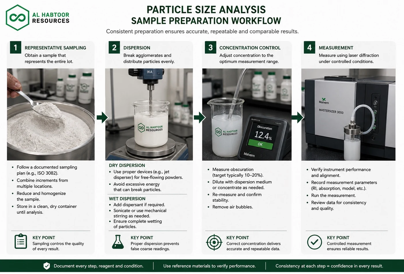
Sample preparation and dispersion
Sample preparation often controls the result more strongly than the instrument itself. Therefore, the laboratory should first obtain a representative sample and then disperse it without either leaving agglomerates intact or breaking primary particles.
- Obtain a representative laboratory sample. Use a suitable splitting method rather than taking material only from the top of a bag.
- Condition the material. Record moisture state when humidity can change agglomeration or flow.
- Select dry or wet dispersion. Choose the route according to material behaviour and the purpose of the test.
- Control energy input. Set air pressure, stirring and sonication at levels that disperse agglomerates without damaging particles.
- Check background and concentration. Confirm instrument cleanliness and a stable measurement window.
- Run replicate measurements. Compare repeats and investigate drifting or multimodal results.
- Retain the procedure. Use the same validated settings for future lot comparisons.
Why two methods can report different particle sizes
Sieve analysis measures whether particles pass through a physical opening. By contrast, laser diffraction calculates an equivalent size from a scattering pattern. Plate-like talc, needle-like particles and irregular mineral grains do not behave like perfect spheres, so the methods may rank the same powder differently.
In addition, sieve analysis usually reports mass fractions, while laser diffraction often reports a volume-equivalent distribution. Therefore, buyers should not convert a laser D90 directly into “mesh passing” unless a validated material-specific correlation supports that conversion.
Use the same method for acceptance that the specification used during product approval. If the buyer needs both coarse residue control and full distribution data, specify both sieve residue and laser diffraction D-values.
How to write a particle size acceptance specification
A strong specification states the method and the limits. For example, “325 mesh” remains incomplete because it does not say whether the supplier means nominal aperture, percentage passing or maximum residue.
| Weak wording | Procurement-ready wording |
|---|---|
| 325 mesh | ASTM E11 No. 325 sieve, 45 um nominal aperture, maximum retained mass stated as a percentage. |
| D50: 10 um | Laser diffraction D50 by volume, target and tolerance stated, with instrument and dispersion procedure identified. |
| Fine powder | D10, D50 and D90 limits plus a maximum coarse residue under the agreed method. |
| 100 percent passing | Minimum passing percentage or maximum residue on a named sieve, tested with a defined sample mass and procedure. |
Buyer specification fields
Particle size COA review checklist
A certificate of analysis should let the buyer reproduce or meaningfully compare the test. Therefore, request clarification when a document reports only “mesh” or one D50 value.
Worked procurement example
A buyer compares two talc lots. Both lots show D50 near 10 um. However, Lot B has a higher D90 and more residue on the 45 um sieve. As a result, Lot B creates more visible specks in a white polymer compound even though the median size appears acceptable.
- D50 alone did not reveal the coarse tail.
- D90 showed the difference in the upper part of the distribution.
- The No. 325 sieve residue confirmed the oversize risk.
- The buyer improved the specification by controlling both D90 and 45 um residue.
Common testing mistakes
| Common mistake | Better approach |
|---|---|
| Using mesh number as an exact diameter | State the standard and nominal aperture. |
| Comparing sieve and laser results directly | Use one validated method or establish a material-specific correlation. |
| Reporting only D50 | Include D10 and D90 or other limits that control fines and coarse particles. |
| Ignoring the distribution basis | State volume, mass or number basis. |
| Changing dispersion pressure or sonication | Use one validated preparation procedure for every lot. |
| Testing an unrepresentative scoop | Use documented sampling and sample splitting. |
| Allowing sieve blinding | Use the appropriate dry or wet method and inspect the sieve condition. |
| Setting a tolerance tighter than repeatability | Confirm method precision before finalising acceptance limits. |
Frequently asked questions
Is 325 mesh always equal to 45 micrometres?
ASTM E11 No. 325 uses a nominal aperture of 45 um. However, a commercial “325 mesh powder” may mean a passing claim, a residue limit or only a product label. Therefore, confirm the standard and percentage retained or passing.
Can mesh be converted directly to D50?
No. Mesh describes a sieve designation, while D50 describes the median of a measured distribution. A powder passing a 45 um sieve can still have many different D50 values.
Why does laser diffraction report a different result from sieving?
The methods measure different physical responses. Sieving classifies by passage through an opening, while laser diffraction calculates an equivalent optical size. Shape, dispersion and reporting basis also affect the result.
Should a specification include both D90 and sieve residue?
Yes, when the application needs a full distribution plus direct control of oversize particles. The two limits answer different questions.
What is the best particle size method for talc?
The best method depends on the application and grade. Laser diffraction provides a broad distribution, while sieve residue can control coarse contaminants. Plate-like shape and dispersion conditions should remain consistent.
Related procurement resources
Technical references
ASTM E11-24 specifies requirements for woven wire test sieve cloth and test sieve construction used to classify materials by particle size.
ISO 13320:2020 provides guidance for instrument qualification and particle size distribution measurement by laser diffraction.
ASTM C371-09(2018) covers wire-cloth sieve analysis of nonplastic ceramic powders, including talc and other mineral materials.
Need a reviewable particle size specification?
Send the target application, required D-values or sieve residue, test method, quantity, packing, destination and document requirements. AHR can coordinate a specification-led mineral supply review.